RedStuff Encoding Algorithm

The RedStuff encoding algorithm used in Walrus is an adaptation of the Twin-Code framework presented by Rashmi et al. [1].

Goals and overview

The goal of the Walrus system is to provide a distributed storage infrastructure, where a decentralized set of entities—the storage nodes—collaborate to store and serve files (blobs of data). When it comes to storage properties, Walrus has 3 key goals:

1. To support extremely high availability and durability of the data.
2. To have low storage overhead compared to full replication, meaning you do not store each blob on every storage node.
3. To gracefully support node failures, and in particular to allow for efficient node recovery (more on this later).

Given these requirements, one good option is to erasure encode the blobs across the storage nodes. At a high level, erasure encoding (or erasure coding) allows you to encode the data into $N$ parts, such that the aggregate size of the $N$blobs is a small multiple of the original blob size, and a subset $k$ of these parts is sufficient to recover the original blob. The next section formalizes these concepts, but note that erasure coding already allows you to achieve goals 1 and 2 above, because:

1. Erasure coding allows you to recover a blob even if $N - k$storage nodes fail, providing high availability and durability.
2. The overall storage overhead is much smaller than for full replication. For a blob of size $S$, the total storage used in the system is $S \cdot c$ instead of $S \cdot N$, where $c \ll N$ is a small constant (4.5 in Walrus's case).

To achieve the third requirement, however, simple erasure coding is insufficient. A failed node that wants to reconstruct its part of the encoding needs to first fetch at least $k$ other parts, reconstruct the blob, and then re-encode its own part. Therefore, the communication overhead for recovery is on the order of the size of the whole blob, $S$. With RedStuff, you can instead reconstruct the encoded part of a failed node by fetching only $O(S/N)$ data, meaning only in the order of the size of the lost part. This achieves goal 3.

Background

This section provides the essential background on the coding schemes used in RedStuff.

Erasure codes

Erasure coding addresses the problem of error correction in the case of bit erasures, where some bits in the message are lost, as in the case of a lossy channel. An erasure code divides a blob (or message) of $S$ bytes into $k$ symbols (bitstrings of fixed length $\sim S/k$), which are then encoded to form a longer message of $N$ symbols, such that the original blob can be recovered from any subset $k'$ of the $N$ symbols. The ratio $k/N$ is called the code rate.

Fountain codes

Fountain codes are a class of erasure codes. The key property of fountain codes is that the encoding process is rateless, meaning the encoder can produce an arbitrary number of encoded parts without knowing the total number of parts that will be produced. This is useful for the RedStuff use case, as it allows you to specify the rate of the encoder. For example, by encoding $f+1$ source symbols into $N$ recovery symbols, you guarantee that any subset of $f+1$ symbols can reconstruct the source. Fountain codes are also extremely efficient as they typically require only XOR operations to encode and decode data.

RaptorQ

RedStuff is based on the RaptorQ fountain code. RaptorQ is one of the fastest and most efficient fountain codes, and has the following properties:

1. It is systematic, meaning the first $k$ symbols of the encoded message correspond to the original message.
2. It is a linear code, meaning the encoding process is a linear transformation of the input symbols, or in other words, the encoded symbols are linear combinations of the input symbols.
3. It is almost optimal, meaning that $k' \approx k$. Specifically, the probability of decoding failure for $k' = k + H$ symbols received is $\lt 1/256^{H+1}$.

RedStuff encoding

An established approach in distributed storage is to use an erasure code to encode blobs of data across multiple storage nodes. By using a $k/N$ rate erasure code for $N$ nodes and $k$ source symbols, the system can tolerate $N - k$ node failures, with just an $N/k$ factor of storage overhead. However, in the case of a node failure, the recovery process is inefficient: the failed node needs to fetch $k$ other parts, reconstruct the blob, and then re-encode its own part. Therefore, the communication overhead for recovery is on the order of the size of the whole blob, $S$.

The Twin-Code framework aims to solve this issue by allowing for efficient node recovery. This section briefly describes how the framework is used in RedStuff. For specific details, refer to the original paper. The RedStuff encoding algorithm is an adaptation of the Twin-Code framework, which allows for efficient node recovery in erasure-coded storage systems.

Consider a scenario in which a blob of data is encoded and stored across $N$ shards—multiple shards can be mapped to the same storage node—in a Byzantine setting. Up to $f$ of the shards can be corrupted by an adversary, with $f \lt 1/3 N$, and the remaining $N - f$ shards are honest.

Encoding and recovery

The RedStuff encoding and recovery process works as follows:

• First, the data blob of size $S$ is divided into symbols and arranged in a rectangular message matrix of up to $N - 2f$ rows and $N - f$ columns of symbols. The number of rows ($n_R$) and columns ($n_C$) is fixed, and determines the symbol size $s$ as follows:

$$s = \left\lceil S / (n_R \cdot n_C) \right\rceil$$

• Then, the columns and the rows of the message matrix are encoded separately with RaptorQ.
  • The primary encoding, performed on columns, expands the $n_R$ symbols of each column to $N$ symbols. The rateless nature of RaptorQ allows you to choose the number of encoded symbols.
  • The secondary encoding, performed on rows, expands the $n_C$ symbols of each row to $N$ symbols.
• $n_R$ is also called the number of primary source symbols, and $n_C$ the number of secondary source symbols. The primary encoding has rate $n_R / N$, and the secondary encoding has rate $n_C / N$.
• The encoded rows and columns are then used to obtain primary and secondary slivers, which are distributed to shards and used for blob reconstruction and sliver recovery:
  • Primary slivers are the rows of the matrix of size $N \times n_C$ obtained with the primary encoding of the message matrix. Each primary sliver is therefore composed of $n_C$ symbols.
  • Secondary slivers are the columns of the matrix of size $n_R \times N$ obtained with the primary encoding of the message matrix. Each secondary sliver is therefore composed of $n_R$ symbols.
• Each shard receives a primary and a secondary sliver, based on the shard number and the row and column numbers of the slivers. See the section on sliver-to-shard mapping for more details.
• The fundamental property achieved with this construction, thanks to the linearity of RaptorQ, is that encoding the primary slivers (as rows) with the secondary encoding and the secondary slivers (as columns) with the primary encoding results in the same $N \times N$ expanded message matrix. This property enables lost sliver recovery:
  • To reconstruct a lost primary sliver, a shard can request $N-f$ symbols from the encodings of the secondary slivers of other shards. Because the primary encoding of secondary slivers results in the symbols for primary slivers, and the secondary encoding has $n_C$ source symbols where $n_C \leq N-2f$, the shard can decode the original primary sliver from the obtained recovery symbols with high probability. See the discussion on recovery probability for more details.
  • The reconstruction of secondary slivers is identical, but with the roles of primary and secondary slivers and encodings inverted.

The following example concretely shows this process.

Worked example

Encoding

Consider a Walrus instance with $N = 7 = 3f + 1$ shards. This means the number of primary source symbols is $N - 2f = 3$, and secondary $N - f = 5$. A blob of size $S = 15 \cdot s$ can therefore be divided into 15 symbols of size $s$, and arranged in the matrix as follows.

$$\left[ \begin{array}{ccccc} s_{0,0} & s_{0,1} & s_{0,2} & s_{0,3} & s_{0,4} \\ s_{1,0} & s_{1,1} & s_{1,2} & s_{1,3} & s_{1,4} \\ s_{2,0} & s_{2,1} & s_{2,2} & s_{2,3} & s_{2,4} \\ \end{array} \right]$$

Then, the primary encoding acts on the columns of the matrix, expanding them such that each column is composed of 4 source symbols and 6 recovery symbols ($s_{i,j}$ indicates source symbols, while $r_{i,j}$ indicates recovery symbols).

$$\left[ \begin{array}{c|c|c|c|c} s_{0,0} & s_{0,1} & s_{0,2} & s_{0,3} & s_{0,4} \\ s_{1,0} & s_{1,1} & s_{1,2} & s_{1,3} & s_{1,4} \\ s_{2,0} & s_{2,1} & s_{2,2} & s_{2,3} & s_{2,4} \\ \color{blue} r_{3,0} & \color{blue} r_{3,1} & \color{blue} r_{3,2} & \color{blue} r_{3,3} & \color{blue} r_{3,4} \\ \color{blue} r_{4,0} & \color{blue} r_{4,1} & \color{blue} r_{4,2} & \color{blue} r_{4,3} & \color{blue} r_{4,4} \\ \color{blue} r_{5,0} & \color{blue} r_{5,1} & \color{blue} r_{5,2} & \color{blue} r_{5,3} & \color{blue} r_{5,4} \\ \color{blue} r_{6,0} & \color{blue} r_{6,1} & \color{blue} r_{6,2} & \color{blue} r_{6,3} & \color{blue} r_{6,4} \\ \end{array} \right]$$

Each of the rows of this column expansion is a primary sliver. For example, $[r_{5,0}, r_{5,1}, r_{5,2}, r_{5,3}, r_{5,4}, r_{5,5}, r_{5,6}]$.

Similarly, the secondary encoding on the rows of the matrix produces the expanded rows.

$$\left[ \begin{array}{ccccccc} s_{0,0} & s_{0,1} & s_{0,2} & s_{0,3} & s_{0,4} & \color{blue} r_{0,5} & \color{blue} r_{0,6} \\ \hline s_{1,0} & s_{1,1} & s_{1,2} & s_{1,3} & s_{1,4} & \color{blue} r_{1,5} & \color{blue} r_{1,6} \\ \hline s_{2,0} & s_{2,1} & s_{2,2} & s_{2,3} & s_{2,4} & \color{blue} r_{2,5} & \color{blue} r_{2,6} \\ \end{array} \right]$$

Each of the columns of this row expansion is a secondary sliver. For example, $[r_{0,6}, r_{1,6}, r_{2,6}]$.

The $i$th sliver pair is composed of the $i$th primary and $i$th secondary slivers. For simplicity, consider that the $i$th sliver pair is stored on shard $i$. The sliver-pair-to-shard mapping section discusses the full mapping.

Thanks to the linearity of RaptorQ, the expansion of:

• the recovery secondary slivers (columns 5 and 6) with the primary encoding, and
• the recovery primary slivers (rows 3, 4, 5, and 6) with the secondary encoding,

results in the same set of symbols, which is essential for recovery. These symbols can be represented as the lower-right quadrant of what is called the fully expanded message matrix.

$$\left[ \begin{array}{ccccc|cc} s_{0,0} & s_{0,1} & s_{0,2} & s_{0,3} & s_{0,4} & r_{0,5} & r_{0,6} \\ s_{1,0} & s_{1,1} & s_{1,2} & s_{1,3} & s_{1,4} & r_{1,5} & r_{1,6} \\ s_{2,0} & s_{2,1} & s_{2,2} & s_{2,3} & s_{2,4} & r_{2,5} & r_{2,6} \\ \hline r_{3,0} & r_{3,1} & r_{3,2} & r_{3,3} & r_{3,4} & \color{blue} r_{3,5} & \color{blue} r_{3,6} \\ r_{4,0} & r_{4,1} & r_{4,2} & r_{4,3} & r_{4,4} & \color{blue} r_{4,5} & \color{blue} r_{4,6} \\ r_{5,0} & r_{5,1} & r_{5,2} & r_{5,3} & r_{5,4} & \color{blue} r_{5,5} & \color{blue} r_{5,6} \\ r_{6,0} & r_{6,1} & r_{6,2} & r_{6,3} & r_{6,4} & \color{blue} r_{6,5} & \color{blue} r_{6,6} \\ \end{array} \right]$$

These symbols do not need to be stored on any node because they can always be recomputed by expanding either a primary or secondary symbol. For example, $r_{4,5}$ can be obtained by:

• the secondary-encoding expansion of the 4th primary sliver: $[r_{4,0}, r_{4,1}, r_{4,2}, r_{4,3}, r_{4,4}, \color{blue} r_{4,5}, r_{4,6}]$, or
• the primary-encoding expansion of the 5th secondary sliver: $[r_{0,5}, r_{1,5}, r_{2,5}, r_{3,5}, \color{blue} r_{4,5}, r_{5,5}, r_{6,5}]$.

Recovery

Consider that shard 3 fails, losing its slivers, and needs to recover them. In the following, the symbols of the lost slivers are highlighted in red (the lower quadrant is never stored).

$$\left[ \begin{array}{ccccc|cc} s_{0,0} & s_{0,1} & s_{0,2} & \color{red} s_{0,3} & s_{0,4} & r_{0,5} & r_{0,6} \\ s_{1,0} & s_{1,1} & s_{1,2} & \color{red} s_{1,3} & s_{1,4} & r_{1,5} & r_{1,6} \\ s_{2,0} & s_{2,1} & s_{2,2} & \color{red} s_{2,3} & s_{2,4} & r_{2,5} & r_{2,6} \\ \hline \color{red} r_{3,0} & \color{red} r_{3,1} & \color{red} r_{3,2} & \color{red} r_{3,3} & \color{red} r_{3,4} & & \\ r_{4,0} & r_{4,1} & r_{4,2} & r_{4,3} & r_{4,4} & & \\ r_{5,0} & r_{5,1} & r_{5,2} & r_{5,3} & r_{5,4} & & \\ r_{6,0} & r_{6,1} & r_{6,2} & r_{6,3} & r_{6,4} & & \\ \end{array} \right]$$

To recover the primary sliver, the node contacts 5 other shards and requests the recovery symbols for the 3rd primary slivers. Because the symbols of the sliver are recovery symbols, the shards need to encode their secondary slivers (highlighted as columns) to obtain them. For example, shards 0, 1, 2, 4, and 6 provide the symbols:

$$\left[ \begin{array}{c|c|c|c|c|c|c} s_{0,0} & s_{0,1} & s_{0,2} & \color{red} s_{0,3} & s_{0,4} & r_{0,5} & r_{0,6} \\ s_{1,0} & s_{1,1} & s_{1,2} & \color{red} s_{1,3} & s_{1,4} & r_{1,5} & r_{1,6} \\ s_{2,0} & s_{2,1} & s_{2,2} & \color{red} s_{2,3} & s_{2,4} & r_{2,5} & r_{2,6} \\ \color{green} r_{3,0} & \color{green} r_{3,1} & \color{green} r_{3,2} & & \color{green} r_{3,4} & & \color{green} r_{3,6}\\ \end{array} \right]$$

To recover the secondary sliver, the node contacts at least 3 other shards to obtain recovery symbols. In this case, the recovery symbols are already part of the primary slivers (highlighted as rows) stored by the other shards, so no re-encoding is necessary. For example, shards 0, 1, and 5 provide the recovery symbols:

$$\left[ \begin{array}{ccccc} s_{0,0} & s_{0,1} & s_{0,2} & \color{green} s_{0,3} & s_{0,4} \\ \hline s_{1,0} & s_{1,1} & s_{1,2} & \color{green} s_{1,3} & s_{1,4} \\ \hline s_{2,0} & s_{2,1} & s_{2,2} & s_{2,3} & s_{2,4} \\ \hline \color{red} r_{3,0} & \color{red} r_{3,1} & \color{red} r_{3,2} & \color{red} r_{3,3} & \color{red} r_{3,4} \\ \hline r_{4,0} & r_{4,1} & r_{4,2} & r_{4,3} & r_{4,4} \\ \hline r_{5,0} & r_{5,1} & r_{5,2} & \color{green} r_{5,3} & r_{5,4} \\ \hline r_{6,0} & r_{6,1} & r_{6,2} & r_{6,3} & r_{6,4} \\ \end{array} \right]$$

In this case, the symbols $s_{0,3}$, $s_{1,3}$, and $s_{2,3}$ are already stored in the primary slivers of shards 0, 1, and 2 directly. Therefore, by requesting these from those shards, shard 3 does not need to decode the symbols to recover its secondary sliver.

Properties and observations

Why the rectangular layout?

The rectangular layout of the message matrix is an optimization for the Byzantine setting. When storing the blob, a client can only await $N - f$ responses, as the remaining $f$ shards might be Byzantine. Yet, $f$ of these $N-f$ might be the Byzantine ones, and the $f$ that did not reply were only slow due to network asynchrony. Therefore, the blob needs to be encoded such that $N-2f$ symbols are sufficient to recover the original blob. This is achieved by the primary encoding.

After the initial sharing phase, the honest shards share and reconstruct the missing slivers from each other. At a steady state, you can always assume that $N - f$ honest shards are in possession of their slivers. The secondary encoding can therefore have a higher rate, $(N-f)/N$, decreasing the storage overhead while maintaining the same fault tolerance properties.

Worst case initial sharing

The following describes how the $N-f$ honest shards can obtain their sliver pairs in the worst case outlined above, where the client shares the slivers with $N-f$ shards, $f$ of which are Byzantine and drop them.

1. The $N-2f$ honest shards receive the sliver pairs.
2. The remaining $f$ honest shards are notified of the stored blob, such as through the chain, and start the process to recover their sliver pairs.
3. First, they recover their secondary slivers, as they can be decoded from $N-2f$ recovery symbols.
4. Then, once all $N-f$ honest shards have their secondary slivers, they can start recovering the primary slivers, which require $N-f$ recovery symbols.
5. All honest shards have their sliver pairs.

Storage overhead

Assume for simplicity that $N=3f+1$. Then, the original blob is divided into roughly $f \cdot 2f = 2f^2$ symbols. The system stores $N \cdot 2f$ primary sliver symbols and $N \cdot f$ secondary sliver symbols, for a total storage of about $9f^2$ symbols.

Therefore, the storage overhead due to RedStuff encoding is about $9f^2 / 2f^2 = 4.5$ times the original blob size.

Differences with the Twin-Code framework

The key modifications in RedStuff, compared to the original Twin-Code framework, are the following:

• RedStuff uses the RaptorQ fountain code for both the Type 0 and Type 1 encoding, as they are called in the paper. The rates are about $(N-2f)/N$ and $(N-f)/N$ respectively. The Type 0 encoding is called the primary encoding, and the Type 1 encoding the secondary encoding.
• The blob is not laid out in a square message matrix, but in a rectangular one. This is an optimization for the specific BFT setting described here.
• Both Type 0 and Type 1 encodings are stored on each shard. These are called slivers, and the 2 together form a sliver pair.

Walrus-specific parameters and considerations

Sliver-pair-to-shard mapping

The previous sections assumed that sliver pair $i$ is stored on shard $i$. In practice, sliver pairs are mapped to shards in a pseudo-random fashion to ensure that the systematic slivers, which contain the original data, are not always stored on the same shard.

This is important because systematic slivers are the most frequently accessed, as they allow you to access the data without any decoding.

The mapping works as follows: each encoded blob is assigned a 32-byte pseudo-random blob ID. This ID is interpreted as an unsigned big-endian integer, and its remainder modulo $N$ is used as a rotation offset, such that sliver pair $i$ is stored on shard $(i + \text{offset}) \mod N$.

Decoding probability and decoding safety limit

As mentioned above, the reconstruction failure probability of the RaptorQ code is $O(256^{-(H+1)})$, where $H$ is the number of extra symbols received. Therefore, in a system with $f$ Byzantine shards, the number of source symbols for the primary encoding should be slightly below $N-2f$, and for the secondary encoding slightly below $N-f$. This ensures that whenever a validity or quorum threshold of messages is received, there is always a positive $H$ for a low failure probability.

The following parameters are used in the encoding configuration:

• $f$, the maximum number of Byzantine shards, is $\lfloor (N-1) / 3 \rfloor$.
• The safety limit for the encoding, $\sigma$, is set as a function of $N$ to ensure high reconstruction probability (see table below).
• The number of primary source symbols (equivalent to the number of symbols in a secondary sliver) is $N - 2f -\sigma$.
• The number of secondary source symbols (equivalent to the number of symbols in a primary sliver) is $N - f -\sigma$.

Currently, $\sigma$ is selected depending on the number of shards as follows:

N shards from	N shards to (incl)	$\sigma$	Prob. failure
0	15	0	0.00391
16	30	1	1.53e-05
31	45	2	5.96e-08
46	60	3	2.33e-10
61	75	4	9.09e-13
76	inf	5	3.55e-15

For example, the following settings apply:

N shards	f	$\sigma$	Num primary	Num secondary
7	2	0	3	5
10	3	0	4	7
31	10	2	9	19
100	33	5	29	62
300	99	5	97	196
1000	333	5	329	662

Blob size limits

In RaptorQ, the size of a symbol is encoded as a 16-bit integer. Therefore, the maximum size of a blob that can be encoded is $2^{16} - 1 = 65535$ bytes. At a minimum, a symbol must be at least 1 byte.

Because the blob is encoded in the rectangular message matrix, the blob size is upperbound by source_symbols_primary * source_symbols_secondary * u16::MAX and lowerbound by source_symbols_primary * source_symbols_secondary. A few examples for the same configurations as above:

N shards	Min blob size	Max blob size	Min encoded blob size	Max encoded blob size
7	15.0 B	983 KB	56.0 B	3.67 MB
10	28.0 B	1.83 MB	110 B	7.21 MB
31	171 B	11.2 MB	868 B	56.9 MB
100	1.80 KB	118 MB	9.10 KB	596 MB
300	19.0 KB	1.25 GB	87.9 KB	5.76 GB
1000	218 KB	14.3 GB	991 KB	64.9 GB

Sliver authentication, blob metadata, and the blob ID

Alongside the efficient encoding performed by RedStuff, shards need to be able to authenticate that the slivers and encoding symbols they receive belong to the blob they requested. This section briefly outlines how this is achieved.

For each sliver, primary or secondary, a Merkle tree is constructed.

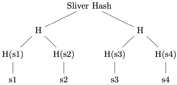
The tree is constructed over all $N$ symbols of the fully expanded sliver. The root node of the Merkle tree (the sliver hash) is included in the metadata for the blob. To prove that a symbol is part of a sliver, the prover supplies the symbol alongside the Merkle path to the root hash, which every node has as part of the metadata.

A Merkle tree over the sliver hashes is then computed to obtain a blob hash. This is computed by concatenating primary and secondary sliver hashes for each sliver pair, and then constructing the Merkle tree over the concatenations ($c_i$ in the figure). This construction reduces the number of hashing operations compared to hashing each sliver Merkle root individually.

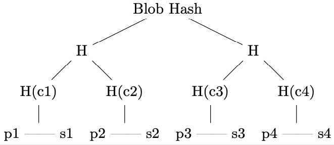
To prove that a sliver is part of a blob, it is sufficient to provide the Merkle path to the root.

Finally, the encoding type tag (representing the RedStuff version or alternative encoding), the length of the blob before encoding, and the Merkle root of the tree over the slivers are hashed together to obtain the blob ID.

Metadata overhead

Each storage node stores the full metadata for the blob. The metadata consists of:

• A 32 B Merkle root hash for each primary and secondary sliver.
• The 32 Bblob ID, computed as above.
• The erasure code type (1 B).
• The length of the unencoded blob size (8 B).

The hashes for the primary and secondary slivers can be a considerable overhead when the number of shards is high. The following table shows the cumulative size of the hashes stored on the system, depending on the number of nodes and shards.

N shards	One node	floor(N/floor(log2(N))) nodes	N nodes
7	448 B	1.34 KB	3.14 KB
10	640 B	1.92 KB	6.40 KB
31	1.98 KB	13.9 KB	61.5 KB
100	6.40 KB	102 KB	640 KB
300	19.2 KB	710 KB	5.76 MB
1000	64.0 KB	7.10 MB	64.0 MB

The cumulative size of the hashes in the case of 1000 nodes (1 node per shard) is 64 KB per node, or 64 MB for a system of 1000 nodes. The number of shards is fixed and constant, while the number of nodes might vary—each node has 1 or more shards—potentially lowering the overhead on the system. The following table shows the ratio between the size of the hashes stored on the system to the minimum and maximum blob sizes, for N=1000 shards and different numbers of nodes (1 node, floor(N/floor(log2(N))) = 111, and 1000).

N = 1000	Total metadata size	Factor min blob	Factor max blob	Factor min encoded blob	Factor max encoded blob
Single node	64.0 KB	0.294	4.48e-06	0.0646	9.85e-07
floor(N/floor(log2(N))) nodes	7.10 MB	32.6	0.000498	7.17	0.000109
N nodes	64.0 MB	294	0.00448	64.6	0.000985

For realistic node counts and small blob sizes, the total metadata overhead can be a multiple of the size of the initial unencoded blob. For larger blob sizes, the overhead is negligible.

---

Reference

[1] K. V. Rashmi, N. B. Shah and P. V. Kumar, "Enabling node repair in any erasure code for distributed storage," 2011 IEEE International Symposium on Information Theory Proceedings, St. Petersburg, Russia, 2011, pp. 1235-1239, doi: 10.1109/ISIT.2011.6033732.